By and large discussions of sample rate are like watching paint dry. Do we really have to get into the details? After all, everyone knows that you only need to sample at twice the frequency of your signal of interest to get good results, right? If you answered “right!” to that last statement, perhaps you should read on. While it’s true that the so-called Nyquist rate of two times the highest signal frequency component is the sample rate required to eliminate alias frequencies, the often overlooked qualifier to this rule is that the signal being digitized must be bandwidth limited at a value equal to half the Nyquist rate. What’s important is not just your frequency of interest, but all the frequencies contained in the signal you digitize and how they compare to the sample rate you’ve chosen. Let’s go back to the basics.
What’s an Alias Frequency?
Webster defines “alias” as an assumed or additional name. For our purposes in data acquisition, we can more accurately define an alias as an assumed or additional frequency. To explore what that means, let’s go to the movies.
You’ve seen it hundreds of times. While watching a movie of a speeding car you look at the car’s wheels and they seem to be rotating impossibly slow, or even rotating backwards. What you’re seeing is an alias frequency caused by a mathematical collision between the fast rotational rate of the car’s wheels and the much slower frame rate of the camera used to record the image. You subconsciously filter this anomaly out of your interpretation of the image because from other frames of reference it’s easy to determine that the car is moving forward at a high rate of speed. But what if you were viewing a movie of just the car’s wheels? In this context, if asked to determine the speed and direction the car was moving you might reach an entirely different, erroneous, and embarrassing conclusion.
Extending the above example, you can think of the camera as the data acquisition system, and the rotating wheels as the signal it’s digitizing. If the sample rate of the data acquisition system is too slow relative to the frequency of the signal, your measurement literally falls apart. You don’t have the convenient frames of reference of the movie. All you have is a conglomeration of changing signal amplitudes versus time. Which are the real ones and which are the aliases? Just like trying to interpret the car’s motion from the movie by watching only the wheels, it’s impossible to know, and there’s too much riding on your measurement to guess.
The Mathematics of Alias Frequencies
We can predict an alias frequency if we know the frequencies of the input signal and the sample rate. Equation (1) shows that alias frequency is a function of the absolute value of the difference between the input signal frequency and the closest integer multiple of the sample rate.
|
fa(N) |
= |
|fin – Nfs| |
(1) |
|
|
fa |
= |
alias frequency | ||
|
fin |
= |
input signal frequency | ||
|
fs |
= |
sample rate | ||
|
N |
= |
an integer greater than or equal to 0 |
Let’s expand upon this equation with some examples. Table 1 is a compilation of various sinusoidal input signal frequencies (fin) sampled at a fixed rate of 1000 Hz and the resulting alias frequencies calculated using equation (1). Constant (N) is an integer that assumes the value necessary to bring the term Nfs closest to the input signal frequency (fin). For example, if the input frequency is 150 Hz and the sample rate is 75 Hz, N equals 2. N moves to 3 if the input signal frequency increases to 188 Hz, because the product of 75 and 3 (225) is closer to 188 than the product of 75 and 2 (150).
As you can see from Table 1, any input signal frequency less than or equal to the Nyquist value of 500 Hz (half the sample rate) is reproduced accurately. Any frequency greater than this value yields an inaccurate alias frequency, even to the extent of reproducing a DC signal when the input frequency is an exact multiple of the sample rate. Clearly, all bets are off when the frequency content of the input signal exceeds one half the sample rate.
Table 1: Alias vs. input frequency at a fixed 1000 Hz sample rate
| Input frequency fin (Hz) |
N | Alias Frequency fa(N) = |fin – Nfs| |
| 500 Hz and less | 0 | fa(0) = |100 – (0)1000| = 100 Hz fa(0) = |200 – (0)1000| = 200 Hz etc. up to and including fin = 500 Hz |
| 501 | 1 | fa(1) = |501 – (1)1000| = 499 Hz |
| 600 | 1 | fa(1) = |600 – (1)1000| = 400 Hz |
| 900 | 1 | fa(1) = |900 – (1)1000| = 100 Hz |
| 1000 | 1 | fa(1) = |1000 – (1)1000| = 0 Hz or DC |
| 1200 | 1 | fa(1) = |1200 – (1)1000| = 200 Hz |
| 2000 | 2 | fa(2) = |2000 – (2)1000| = 0 Hz or DC |
| 2600 | 3 | fa(3) = |2600 – (3)1000| = 400 Hz |
| 4125 | 4 | fa(4) = |4125 – (4)1000| = 125 Hz |
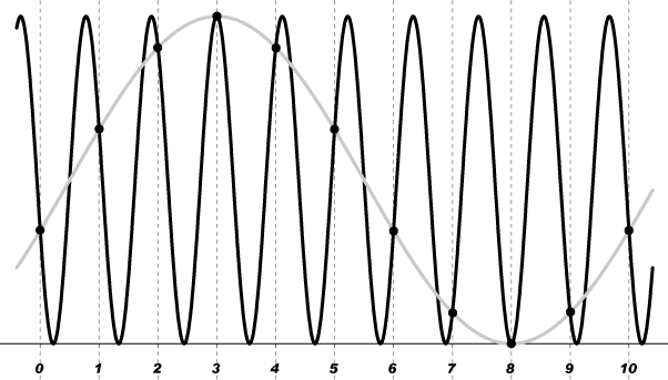
And what does an alias frequency look like? That’s the insidious thing. It looks just like real data. If we were to acquire data in the manner described in Table (1) when fin is equal to 900 Hz we’d see the gray 100 Hz alias waveform shown in Figure 1 instead of the black 900 Hz waveform that was actually connected to our data acquisition system. Aside from the lower frequency, can you tell the difference between the real signal and the ghost? To further complicate things most of us don’t run around acquiring pure sine waves. The typical waveform is a complex assemblage of many frequencies, and a recorded waveform that’s aliased might look perfectly reasonable but lead you to exactly the wrong conclusions.

Figure 1 – A 900 Hz waveform (black) produces an aliased, 100 Hz waveform (gray) when under-sampled at 1000 Hz
What’s the Solution?
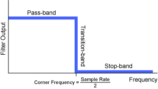
Circling back around to where this application note began, we can satisfy the Nyquist sample rate criterion of two times the maximum signal frequency of interest only if we ensure that no other frequency components higher than this limit exist in the signal. Unless we have a high degree of confidence in the frequency content of the signal source, the only way to achieve this condition is to apply the input signal to a low pass anti-aliasing filter before digitizing it. An in-depth discussion of anti-alias filters is beyond the scope of this application note, but their salient characteristics can be summarized as follows:
- Low-pass design
- The corner frequency is selected to be at your maximum frequency of interest (i.e. at half of the sample rate)
- Steep transition-band roll-off from the pass-band to the stop-band.
Figure 2 is a graphical representation of the ideal anti-alias filter described above. Note that the ideal perpendicular shape of the transition-band is not possible in actual filter design, producing instead a roll-off with some negative slope. This reality forces a compromise in the form of either a lower corner frequency or a higher sample rate. For example, the human ear can respond to frequencies up to 20 kHz. If an anti-alias filter that adheres to the ideal was possible, music could be digitized using a sample rate of 40 kHz. However the standard rate of 44.1 kHz reflects both the reality of less than ideal filter implementations and the desire to maintain a full 20 kHz response.
Do You Really Need an Anti-alias Filter?
There is a cross section of pundits in this field who insist that data acquired without an anti-alias filter are useless. These same people would probably insist that you wear your seatbelt just to pull your car into your garage because “seatbelts save lives.” The fact is that much of the data that’s acquired in day-to-day measurements don’t require an anti-alias filter to yield perfectly accurate and actionable results, and that’s why the vast majority of data acquisition and data logger instruments don’t build one into each measurement channel. Anyone who disagrees with this statement should ask himself or herself if a filter is needed to measure battery voltage – pure 0 Hz. If not, then we’ve at least cracked the door to compromise and we can open it further to include the measurement of other DC or near DC signals: temperature, humidity, DC current, flow, pressure, load, torque, spectrograms, GSR, smooth and skeletal muscle baths, etc. Then what about signals where the frequency content is well defined and contained: 50/60/400 Hz voltages and currents, blood pressures and flows, and even some bio-potentials like ECG and EMG? We’re starting to cover a lot of measurement territory without the need for a filter. There are many more examples, but filters do have their place.
Accelerometer-based measurements are the best examples of where anti-alias filters are a virtual necessity. Most piezoelectric accelerometers have a frequency response in excess of 15 kHz. Although your frequency of interest may be much lower than that (e.g. 40 Hz motor rumble because of bearing wear) you cannot ignore the fact that the sensor can and will pass higher frequencies. If you’ve read this far, you should know that just because you’re not interested in frequencies above 40 Hz doesn’t mean that you only have to sample at 80 Hz or so if the sensor can pass frequencies orders of magnitude higher.
You Probably Need to Oversample
We’ve seen thus far that a bandwidth-limited input signal that is sampled at a rate of at least twice the corner frequency of the anti-alias filter allows the frequency content of the input signal to be reproduced. This is great if you’re only interested in the frequency content of the system under test, and there are applications where this is the extent of the analysis. Going back to the accelerometer example, you really don’t care what the waveform looks like because it’s the frequency spectrum that conveys the presence and frequency of motor rumble. But for other applications where the waveform shape does convey information, good luck extracting that from two samples per cycle. Referring to the 100 Hz, aliased waveform of Figure 1, you can’t even remotely reconstruct that sine wave with only two points. Whenever you need accurate waveform reproduction your only recourse is to oversample at a rate beyond Nyquist’s 2 times minimum, typically 10 times or more. Assuming that you have accurately accounted for the frequency content of your signal and eliminated the potential for alias frequencies, the actual multiple you choose is determined by personal preference.
Thanks for reading.


 View Cart
 sales@dataq.com
 330-668-1444